Workshop fNIRS 2022
This page corresponds the mini-course given at the fNIRS conference in 20222. More information here: https://fnirs2022.fnirs.org/educational/mini-courses/minicourse-20/
- Edouard Delaire, Physics Department and PERFORM Center, Concordia University, Montreal, Canada
- Thomas Vincent, EPIC center, Montreal Heart Institute, Montreal, Canada
- Zhengchen Cai, Physics Department and PERFORM Center, Concordia University, Montreal, Canada
- Christophe Grova, Physics Department and PERFORM Center, Concordia University, Montreal, Canada
- Hardware: a basic recent laptop should be fine.
- An internet connection. A dedicated wifi connection will be available on site for the participants of the workshop.
- Operating system: Linux, windows or Mac OS. Everything should work on all systems though we recommend using Linux since more tests have been done with it.
- Disk space: the full installation with dependencies and sample data should take no more than 4Gb. Some space can be freed by cleaning the CPLEX dependency (saves ~3Gb).
-
Matlab: version > R2015b is recommended.
The Matlab Curve Fitting Toolbox is required to perform motion correction. If you don't have it, you may skip this step in the first tutorial. The provided data do not contain too much movement. - Before attending the workshop: Please complete the following Setup section.
If Brainstorm is already installed, update to the latest version (Menu bar: Update > Update Brainstorm).
For a new installation, Brainstorm requires a user to be registered in order to download it. This allows their development team to track their usage. Consult Brainstorm tutorial for instruction on how to download Brainstorm
For the first time it runs, brainstorm asks to specify a database folder. This will be the place where all the data imported by brainstorm will go. Create a folder named brainstorm_db in your Documents folder and specify it as your main brainstorm database. Then, the main brainstorm interface will be displayed.
No prior knowledge of brainstorm is mandatory for the current workshop session which should cover the basics. However, if one wishes to get familiar with brainstorm features, we refer to the brainstorm tutorials page.
Important for mac users: If the right-click doesn't work anywhere in the Brainstorm interface and you cannot get to see the popup menus in the database explorer, try to change the configuration of your trackpad in the system preferences and enable left-click. Alternatively, connect a standard external mouse with two buttons. Some Apple pointing devices do not interact very well with Java/Matlab.
CPLEX is a set of tools to perform functional optimization edited by IBM. It is used here to solve the integer programming problem during the optimal montage computation (last tutorial of this workshop).
For license concerns, we cannot bundle the CPLEX library within NIRSTORM. One can purchase a free copy of CPLEX if they are students or academics.
For this tutorial, download CPLEX 12.10.
To download CPLEX :
- Visit http://ibm.biz/CPLEXonAI and create an account using your institutional email
- Once you are connected; go down the page and click on software and then ILOG CPLEX Optimization Studio and click on download. A new page will open
- In the search options, select text, and write: "IBM ILOG CPLEX Optimization Studio V12.10 Multiplatform Multilingual eAssembly"
- Download "IBM ILOG CPLEX Optimization Studio V12.10 for X Multiplatform Multilingual" where X is your operating system (eg. Windows, Linux, MacOs)
- For MacOs, install CPlex.
- For Linux, and Windows, unzip the file in your Documents
Finally, add the path to the CPLEX Matlab bindings to the Matlab path: go to the "Home" tab, click "Set path" (yellow folder icon) then click on "Add with subfolders" and select the folder of the CPLEX Matlab bindings.
In Mac, this file is in your application folder.
If you cannot get a working version of CPLEX, let us know during the workshop and we'll try to help you.
Using Brainstorm plug-in system, download the following plugins :
- NIRS > NIRSTORM
- NIRS > MCXLAB-cl
- SPM12
- Inverse > Brainentropy
The tutorial is separated into three modules
- Module 1: Channel-space analysis: extraction of the motor response
- Module 2: Source-space analysis: Reconstruction of the motor response on the cortical surface
- Module 3: Optimal montage computation
- One subject, one run of 19 minutes acquired with a sampling rate of 10Hz on a CW fNIRS Brainsight device (Rogue-Research Inc., Montreal, Canada)
- Finger tapping task: 20 blocks of 10 seconds each, with a rest period of 30 to 60 seconds
- 3 sources, 15 detectors, and 1 proximity detector
- 2 wavelengths: 685nm and 830nm
- 3T MRI anatomy processed by FreeSurfer 5.3.0 and SPM12
The total disk space required after data download and installation is ~1.3Go. The size is quite large because of the optical data which are required for the computation of the forward model. The dataset can be downloaded from: https://drive.google.com/file/d/1b8AYRc7_4vIxdFCpMs5QCri_kTcCK-G7/view?usp=sharing .
For the optimal montage, download Colin27 template, to do so, execute the following command in Matlab : nst_bst_set_template_anatomy('Colin27_4NIRS_Jan19', 0, 1)
** Licence ** This tutorial dataset (NIRS and MRI data) remains proprietary of the MultiFunkIm Laboratory of Dr Grova, at PERFORM centre, Concordia University, Montreal. Its use and transfer outside the Brainstorm tutorial, e.g. for research purposes, is prohibited without written consent from our group. For questions please contact Christophe Grova: [email protected]
This tutorial illustrates how to estimate the NIRS response to a finger-tapping task at the sensor level and to perform statistical analysis using a general linear model (GLM) at the subject level.
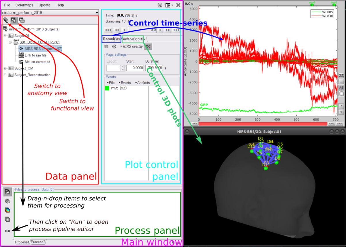
Here is a cheat sheet on the main Brainstorm features that will be used during the tutorials:
First, start by creating a new protocol called For more details, please consult Brainstorm tutorials #1-5
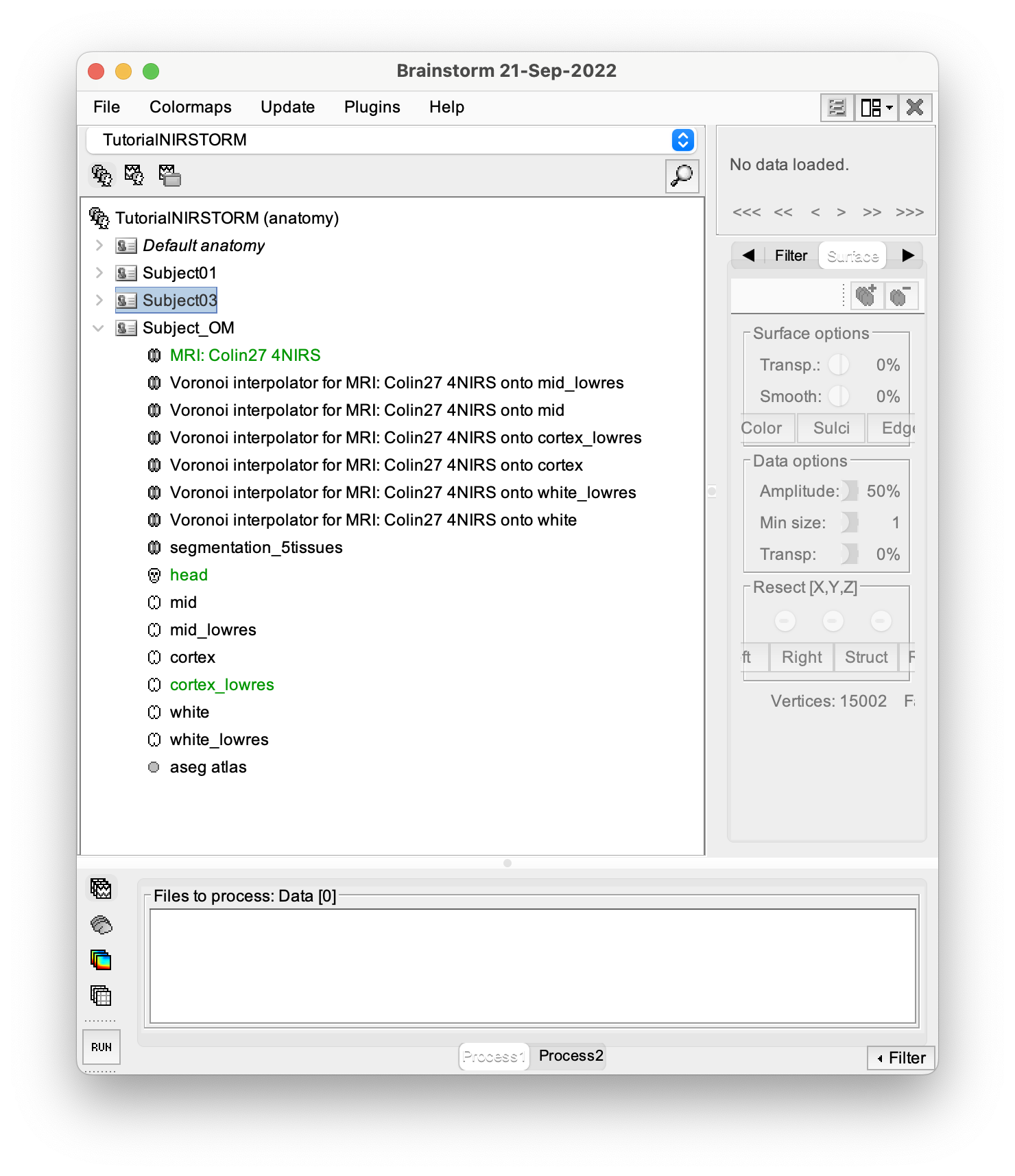
To ensure, that we are all working on the same dataset, we prepared a subject with the anatomy already imported. To import this subject in Brainstorm, click on File > load protocol > import subject from zip and then select TutorialNIRSTORM_Subject01.zip under the bst_db folder. For the rest of the tutorial, make sure that the remeshed head and the mid-cortical surface are selected as the default surface. They should appear in green as in the following picture.
Your Brainstorm database should look like this:

The functional data used in this tutorial was produced by the Brainsight acquisition software and is available in the Functional folder. It contains the following files:
-
fiducials.txt: the coordinates of the fiducials (nasion, left ear, right ear). The positions of the Nasion, LPA, and RPA have been digitized at the same location as the fiducials previously marked on the anatomical MRI. These points will be used by Brainstorm for the registration, hence the consistency between the digitized and marked fiducials is essential for good results. -
optodes.txt: the coordinates of the optodes (sources and detectors), in the same referential as in fiducials.txt. Note: the actual referential is not relevant here, as the registration will be performed by Brainstorm afterward. -
tapping.nirs: the NIRS data in a Homer-based format. Note: The fields ''SrcPos'' and ''DetPos'' will be overwritten to match the given coordinates in "optodes.txt"
To import this dataset in Brainstorm:
- Go to the "functional data" view of the protocol.
- Right-click on Subject 01 > '''Review raw file
- Select file type '''NIRS: Brainsight (.nirs)
- Select file
tapping.nirs - Note: the importation process assumes that the files optodes.txt and fiducials.txt are in the same folder as the .nirs data file.
In the same way, as in the tutorial Channel file / MEG-MRI coregistration, the registration between the MRI and the NIRS is first based on three reference points Nasion, Left and Right ears. It can then be refined with either the full head shape of the subject or with manual adjustment.
-
The initial registration is based on the three fiducial points that define the Subject Coordinate System (SCS): nasion, left ear, and right ear.
-
These same three points have also been marked before the acquisition of the NIRS recordings. The person who recorded this subject digitized their positions with a tracking device (here Brainsight). The position of these points is saved in the NIRS datasets (see fiducials.txt).
-
When the NIRS recordings are loaded into the Brainstorm database, they are aligned on the MRI using these fiducial points: the NAS/LPA/RPA points digitized with Brainsight are matched with the ones we placed in the MRI Viewer.
-
To improve this registration, we recommend our users to always digitize additional points on the head of the subjects: around 100 points uniformly distributed on the hard parts of the head (skull from nasion to inion, eyebrows, ear contour, nose crest). Avoid marking points on the softer parts (cheeks or neck) because they may have a different shape when the subject is seated on or lying down in the MRI. More information on digitizing head points.
To import the head points, right-click on NIRS-BRS channels (104) and select Digitalized head points > add points. Then select the file called head points in the Functional folder with the format EEG: ASCII, name,XYZ(.). then Right click on NIRS-BRS channels (104) and select Digitalized head points > Remove points below nasion, finally Right click on NIRS-BRS channels (104) and select `MRI registration > Refine using head points (ignore 0% of the headpoints)
The following figure showing the coregistration between the subject anatomy and the montage should appear :
 .
.
Right-click on Link to raw file under the tapping condition and use NIRS > Display time series. It will open a new figure with superimposed channels.

The default temporal window may be limited to a couple a seconds. To actually see the whole time series, in the main brainstorm window -- right panel, go to the "Record" tab, and change "Start" to 0 and "Duration:" to 709.3s (you can see the total duration at the top right of the brainstorm main window).
If coloring is not visible, right-click on the figure the select "Montage > NIRS Overlay > NIRS Overlay" Indeed, brainstorm uses a dynamical montage, called ''NIRS Overlay,'' to regroup and color-code nirs time-series depending on the wavelength (red: 830nm, green:686nm). The signals for a given pair of source and detectors are also grouped when using the selection tool. So clicking one curve for one wavelength will also select the other wavelength for the same pair.
To isolate the signals of a selected pair, the default behaviour of brainstorm can be used by pressing ENTER or right-click on the figure then "Channel > View selected". However, the NIRS overlay dynamic montage is not activated in this case (will be fixed in the future).
During the experiment, the stimulation paradigm was run using E-Prime and sent triggers through the parallel port to the acquisition device. These stimulation events are then stored as a box signal in channel AUX1: values above a certain threshold indicate a stimulation block.
To view the auxiliary data, right-click on Link to raw file and select NIRS_AUX > Display time series
In the event panel, click on file > Read events from channel and use the following options:

Double click on Àux1and rename it tapping. Later in the tutorial, we will need to have access to the duration of the task, to specify it, first duplicate the event using Events > Duplicate groups, and rename it tapping_ext. Finally use Events > Convert to extended events and specify 0ms for the time to include before the event and 10000ms for the time to include after the event (i.e. 10s duration blocks of our tapping data, the default time unit in Brainstorm is the millisecond).
Drag and drop the file Link to raw to the process box, and click run. You can create a pipeline by adding process one after the other that will get executed sequentially.
Add the following process to your pipeline
- NIRS > Pre-process > Detect Bad channels
- NIRS > dOD and MBLL > raw to delta OD
- Pre-process > Band-pass filter
- NIRS > Pre-process > Remove superficial noise
- NIRS > dOD and MBLL > MBLL delta OD to delta [HbO], [HbR] & [HbT]
For the process, use the following parameters :

then click on Run. The following report should appear :

The goal is to get the response elicited by the motor paradigm. For this, we perform window-averaging time-locked on each motor onset while correcting for baseline differences across trials.
The first step is to split the data into chunks corresponding to the window over which we want to average. The average window is wider than the stimulation events: we'd like to see the return to baseline / undershoot after stimulation.
Right-click on "Link to raw file | band(0.01-0.1Hz)| SSC (mean): [0.000s,1123.200s]" under the condition "tapping_dOD_Hb" and use Import in database using the following parameter :

Ensure that "Use events" is checked and that the tapping events are selected. The epoch time should be: -10000 ms to 30000 ms. This means that there will be 10 seconds prior to the stimulation event to check if the signal is steady. There will also be 30 seconds after the stimulation to check the return to baseline / undershoot. In the "Pre-processing" panel, check "Remove DC offset" and use a Time range of -10000ms to 0 ms. This will set a reference window prior over which to removing chunk offsets. All signals will be zero-centered according to this window. Finally, ensure that the option "Create a separate folder for each event type" is unchecked".
This will create 20 tapping files corresponding to each trial that you can review individually. A trial showing excessive motion can be discarded by right-clicking on it and using reject trial. In our example, we want to reject the first trial as it is contaminated y the transient effect of the filter (presence of the event transient_bandpass)
To compute the average response, Drag and drop the 20 files into the process box, it will show `tapping (20 files) [19]. 19 means that only 19 files out of the 20 will be used (since we rejected 1 trial).
Click on run, and select the process Average > Average files. Use the function Arithmetic average + Standard error and use the option Keep all event markers from the individual epochs.
You can then visualize the average by inspecting the file AvgStderr: tapping (19)
Note on the preprocessing: Short-channel regression should not be done twice. If you use the GLM, we recommend performing the short-channel regression inside the GLM module.
Drag and drop the file "Link to raw file | band(0.01-0.1Hz)" from the condition tapping_dOD and create the following pipeline :
- NIRS > dOD and MBLL > MBLL delta OD to delta [HbO], [HbR] & [HbT]
- NIRS > GLM > 1st level design and fit
- NIRS > GLM > 1st level contrast
- NIRS > GLM > contrast t-test

This tutorial illustrates how to perform NIRS reconstruction: estimate NIRS signals in the cortical layer that was at the origin of the signals measured in the channel space on the scalp.
This module is composed of two steps :
- The computation of the forward model
- The computation of the inverse solution using Minimum Norm Estimate (MNE) and Maximum Entropy on the Mean (MEM)
The goal is to get the change in $ \Delta Od $ elicited by the motor paradigm. Doing the same steps, as for windows averaging on after the MBLL, we can compute the evoked response on the $ \Delta Od $ data.
Right-click on "Link to raw file | band(0.01-0.1Hz)| SSC (mean): [0.000s,1123.200s]" under the condition "tapping_dOD" and use Import in database using same parameter as before.
The NIRS reconstruction process relies on the so-called forward problem which models light propagation within the head. It consists in generating the sensitivity matrix that maps the absorption changes along the cortical region to optical density changes measured by each channel (Boas et al., 2002). Akin to EEG, this is called here the head model and is already provided in the given data set (this is the item NIRS head model).
This will create 20 tapping files corresponding to each trial that you can review individually. A trial showing excessive motion can be discarded by right-clicking on it and using reject trial. In our example, we want to reject the first trial as it is contaminated y the transient effect of the filter (presence of the event transient_bandpass)
To compute the average response, Drag and drop the 20 files into the process box, it will show `tapping (20 files) [19]. 19 means that only 19 files out of the 20 will be used (since we rejected 1 trial).
The anatomy preprocessed from FreeSurfer should already be imported from Module 1. In order, to compute the forward model, we need to compute the Voronoi interpolator. For the rest of the tutorial, make sure that the remeshed head and the mid-cortical surface are selected as the default surface. They should appear in green as in the following picture.
- The Voronoi interpolator: interpolators project volumic data onto the cortical mid surface. It will be used to compute NIRS sensitivity on the cortex from volumic fluence data in the MRI space. It has been computed using the nirstorm process "Compute Voronoi volume-to-cortex interpolator".
The next step is to compute the Voronoi interpolator. This step will create an interpolation matrix from the MRI volume to the selected cortical surface. Before computing both the T1 MRI, and the mid-surface are selected (they should be highlighted in green in the next figure).
To compute the Voronoi interpolator, click on run, without any file in the process box, and under NIRS > Sources, select Compute Voronoi volume-to-cortex interpolator. Then select the subject, and use the Grey matter masking option.
The anatomy view should now look like this:

Fluences data reflecting light propagation from any head vertex can be estimated by Monte Carlo simulations using MCXlab developed by (Fang and Boas, 2009). Sensitivity values in each voxel of each channel are then computed by multiplication of fluence rate distributions using the adjoint method according to the Rytov approximation as described in (Boas et al., 2002). Nirstorm can call MCXlab and compute fluences corresponding to a set of vertices on the head mesh. To do so, one has to set the MCXlab folder path in Matlab and has a dedicated graphics card since MCXlabl is running by parallel computation using GPU. See the MCXlab documentation for more details.
You need to load the plugin called MCXlab-cl (or MCXlab-cuda if your GPU supports CUDA)
To compute the forward model, put the file AvgStderr: tapping (19) from the condition tapping_dOD in the process box and use the process NIRS > Sources > compute fluences. After selecting your subject name, and clicking on Edit, the following panel should appear:

The main parameters to consider are :
- Segmentation label: the label used to describe the tissues in your segmentation file. Here scalp (labeled as 5), skull (labeled as 4), CSF (labeled as 3), grey matter (labeled as 2), and white matter (labeled as 1)
- The GPU / CPU used for the simulation and the number of photons to simulate.
- The output folder in which the fluences will be stored.
For this workshop, we pre-computed the fluences and stored them in the Fluences folder.
Finally, compute the forward model, using NIRS > sources > Compute head model from fluence.
Under path, copy the path to the fluence folder (eg /Users/edelaire1/Desktop/workshop-2022/Fluences) and leave the rest of the options as shown in the following figure :

The visualize the current head model, use NIRS > sources > Extract sensitivity surfaces from head model
If selected, the option Normalize sensitivity map will convert the sensitivity map to a normalized map on the log-scale. (EG normalized sensitivity = log( sensitivity / max (sensitivity) )
Two maps will be created per wavelength : Summed sensitivities and Sensitivites.
Summed sensitivities provide an overall insight of the cortical sensitivity of the NIRS montage by summing the sensitivity of every channels. Sensitivites provide information about the sensitivity of every channel individualy. We used a trick to store pair information in the temporal axis. The two first digits of the time value corresponding to the detector index and the remaining digits to the source index. So time=101 corresponds to S1D1. With the same logic, time=210 is used for S2D10. Note that sometimes indexes do not correspond to any source-detector pair and the sensitivity map is then empty at these positions. The following figure shows the summed sensitivity profile of the montage (bottom) and the sensitivity map of one channel S2D6 (top).

Reconstruction amounts to an inverse problem which consists in inverting the forward model to reconstruct the cortical changes of hemodynamic activity within the brain from scalp measurements (Arridge, 2011). The inverse problem is ill-posed and has an infinite number of solutions. To obtain a unique solution, regularized reconstruction algorithms are needed. The two algorithm available in NIRSTROM are Minimum Norm Estimate (MNE) and Maximum Entropy on the Mean (MEM)
Minimum norm estimation (MNE) is one of the most widely used reconstruction method in NIRS tomography. It minimizes the l2-norm of the reconstruction error along with Tikhonov regularization (Boas et al., 2004).
Drag and drop "AvgStd FingerTapping (20)" into the process field and press "Run". In the process menu, select "NIRS > Source reconstruction - wMNE".
The parameters of this process are:
- Depth weighting factor for MNE: 0.3
These factors take into account that NIRS measurements have larger sensitivity in the superficial layer and are used to correct for signal sources that may be deeper. - Compute the noise covariance: If selected, compute the noise covariance matrix according to the baseline window defined below. The covariance matrix is defined using a diagonal matrix with one value per channel. Otherwise, the identity matrix will be used to model the noise covariance.

Note that the standard L-Curve method (Hansen, 2000) was applied to optimize the regularization parameter in MNE model. This actually needs to solve the MNE equation several times to find the optimized regularization parameter. Reconstruction results will be listed under "AvgStd FingerTapping (19)". The reconstructed time course can be plotted by using the scout function as mentioned in MEM section.

The MEM framework was first proposed by (Amblard et al., 2004) and then applied and evaluated in Electroencephalography (EEG) and Magnetoencephalography (MEG) studies to solve inverse problem for source localization (Grova et al., 2006; Chowdhury et al., 2013). Please refer to this tutorial for more details on MEM.
To run the NIRS reconstruction using cMEM:
- Drag and drop AvgStd FingerTapping (19) into the process field
- Click "Run". In the process menu, select NIRS > Compute sources: BEst.

The parameters of this process are:
-
Depth weighting factor for MNE and Depth weighting factor for MEM: 0.3
These factors take into account that NIRS measurements have larger sensitivity in the superficial layer and are used to correct for signal sources that may be deeper. MNE stands for "Minimum Norm Estimation" and corresponds to a basic non-regularized reconstruction algorithm whose solution is used as a starting point for MEM. -
Set neighborhood order automatically: selected?
This will automatically define the clustering parameter (neighborhood order) in MEM. Otherwise please make sure to set one in the MEM options panel during the next step.
Clicking on "Edit" opens another parameter panel:

- Select cMEM in the MEM options panel. Keep most of the parameters by default and set the other parameters as:
- Data definition > Time window: 0-30s which means only the data within 0 to 30 seconds will be reconstructed
- Data definition > Baseline > within data checked, with Window: -10 to -0s which defines the baseline window that will be used to calculate the noise covariance matrix.
- Clustering > Neighborhood order: If Set neighborhood order automatically is not checked in the previous step, please give a number such as 8 for NIRS reconstruction. This neighborhood order defines the region growth-based clustering in the MEM framework. Please refer to this tutorial for details. If Set neighborhood order automatically is checked in the previous step, this number will not be considered during MEM computation.
Click "Ok". After less than 10 minutes, the reconstruction should be finished.
Unfold AvgStd FingerTapping (19) to show the MEM reconstruction results. Double-click on the files cMEM sources - HbO and cMEM sources - HbR to review the reconstructed maps,
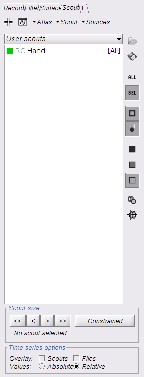
To show the reconstructed time courses of HbO/HbR, one needs to define a region where to extract these time courses.
Switch to the "scout" tab in the view control panel. Then click on the scout "Hand". Under "time-series options" at the bottom, use "Values: Relative". Then in the "Scout" drop-down menu at the top of the tab, select Set function to "All". Finally, click on the wave icon to display the time courses.
By repeating the same process for both HbO and HbR, the results should look like this:

This process is part of the experiment planning, taking place before the acquisition, where the experimenter wants to define where to place the optode on the scalp. Usually, a NIRS montage has limited coverage over the head and hence optodes are placed specifically on top of a predefined target cortical region of interest (ROI). However, due to the non-trivial light propagation across head tissues as well as the complex cortical topology, the optode placement cannot be optimally based solely on a pure geometrical criterion.
Here, the computation of the optimal NIRS montage consists of finding the set of optode coordinates whose sensitivity to a predefined region of interest is maximized (Machado et al., 2014; Pellegrino et al., 2016).
To achieve this, this process requires:
- an anatomical MRI,
- pre-computed fluence data,
- a target ROI, either on the cortex or on the scalp.
For ease of configuration, the current tutorial relies on the Colin27 template adapted to NIRS (included in the workshop sample data). Indeed, fluence maps have already been pre-computed for this anatomy so that one can directly run the optimal montage process without going through the forward model computation. However, the most accurate results are obtained when using the subject-specific MRI. The current procedure can be straightforwardly transposed to any MRI.
Note that fluence data available in the downloaded sample data cover only the region of interest considered here. It amounts to around 1/10th of the head and data takes ~500Mb. In order not to have to download the whole head data (~6 Gb), NIRSTORM provides an on-demand fluence download system (specifically for the Colin27 template).
It will download only the fluence data required to cover the considered region if they are not already available on the local drive (in .brainstorm/defaults/nirstorm/fluence/MRI__Colin27_4NIRS).
- Create a new subject, called "Subject_OM", with the default set-up
- Go to the anatomy view, right-click on Subject_OM and select "Use template > Colin27_4NIRS_Jan19". To download the Colin27 template, to do so, execute the following command in Matlab : nst_bst_set_template_anatomy('Colin27_4NIRS_Jan19', 0, 1)
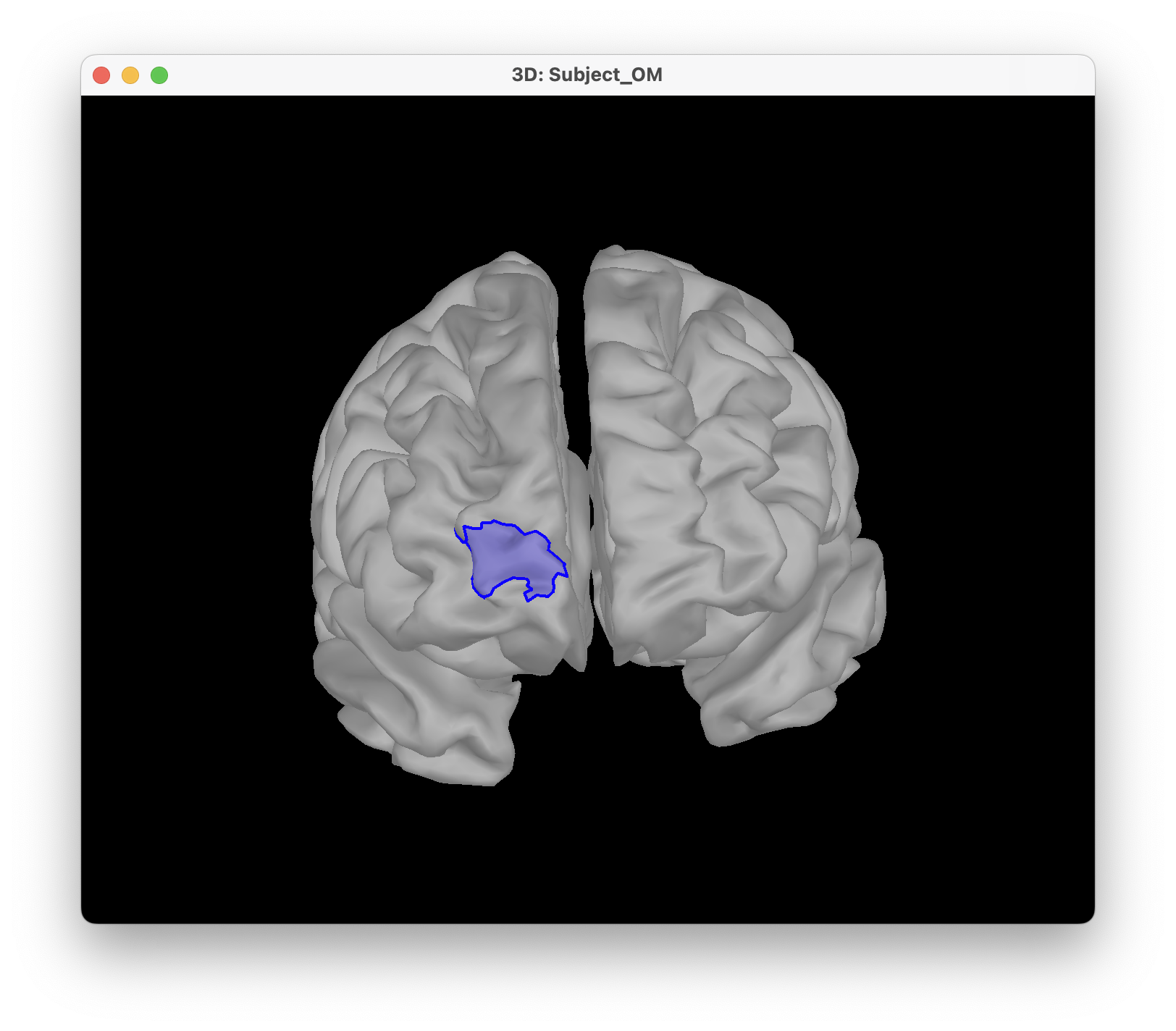
For ease of reproducibility, the ROI definition is atlas-based. For this tutorial, we will target the frontopolar gyrus. For that, we will target the region labeled "RPF G_and_S_transv_frontopol" from the Destrieux atlas. To visualise the region,
- Open the mid cortical mesh by double-clicking on it in the anatomical view of Subject_OM
- Select the scout panel and use the drop-down menu to show the Destrieux atlas
- Select the scout defining the bottom of the frontopolar gyrus, labeled "RPF G_and_S_transv_frontopol".
The optimal montage works by searching for the best possible layout of optode pairings within a given region on the head mesh (search space). Each vertex in this region is a candidate holder on which an optode (source or detector) can be placed. A montage is best if it maximizes the optical sensitivity over a pre-defined cortical region of interest.
Without any file in the process panel, click run and then NIRS > Source > Compute optimal montage. Select the subject and click on Edit. The following figure should appear :
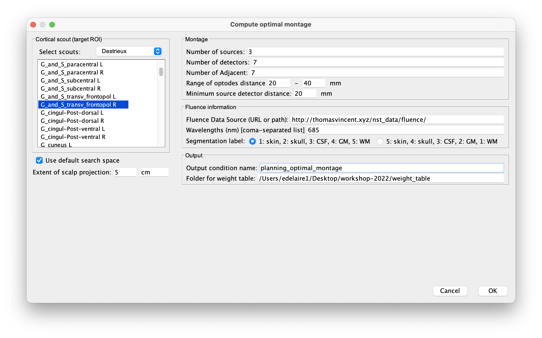
Here are the process parameters to fill in, along with some explanation about them:
-
Cortical scout (target ROI), select Destrieux atlas and G_and_S_transv_frontopol R.
-
Search space : To avoid the explicit definition of the head region (search space), we will use the option 'use default search space' which constructs the head scout by projecting the target cortical scout onto the head mesh. Use 3 cm for the extent of scalp projection. Alternatively, note that the head scout could be given explicitly by selecting the head scout.
Montage :
-
Number of sources: 4
Maximal number of sources in the optimal montage. The actual number in the resulting montage may be lower. -
Number of detectors: 8
Maximal number of detectors in the optimal montage. The actual number in the resulting montage may be lower. -
Number of adjacent: 2
Minimal number of detectors that must be seen by any given source. -
Range of optodes distance: 20 - 40 mm
Minimal and maximal distance between two optodes (source or detector). This applies to source-source, detector-dectector, and source-detector distances. -
Minimum source detector distance: 20 mm
Minimal distance between a source and a detector.
Fluence information
-
Fluence Data Source (URL or path): enter the path to the fluences. For colin27, specify "http://thomasvincent.xyz/nst_data/fluence/" and the necessary fluences will be automatically downloaded.
-
Wavelength (nm): 685
The wavelength of the fluence to load and which will be used to compute the optical sensitivity to the target cortical ROI. Note that optimal montages vary only very slightly across wavelengths. Hence we don't need to use the two actual wavelengths used during acquisitions. This saves some computation time! -
**Segmentation label **: the label used to describe the tissues in your segmentation file. Here scalp (labeled as 1), skull (labeled as 2), CSF (labeled as 3), grey matter (labeled as 4), and white matter (labeled as 5)
Output:
-
Output condition name: Optimal_Montage_frontal
The name of the condition (output functional folder) which will contain the computed montage. -
** Folder for weight table ** : Folder to save the optical sensitivity to the target cortical ROI.
The optimal montage computations comprise the following steps with their typical execution time in brackets:
-
Mesh and anatomy loading [< 10 sec]
-
Loading of fluence files [< 1 min]
Fluence files will be first searched for in the folder .brainstorm/default/nirstorm/fluence. If not available, they will be requested from the resource specified previously (online here).
-
Computation of the weight table (summed sensitivities) [< 3 min]
For every candidate pair, the sensitivity is computed by summation of the normalized fluence products over the cortical target ROI. This is done only for pairs fulfilling the distance constraints. This step if skipped if the weight table folder is specified and a weight table was already pre-computed.
-
Linear mixed integer optimization using CPLEX [~ 5 min]
This is the main optimization procedure. It explores the search space and iteratively optimizes the combination of optode pairings while guaranteeing model constraints.
-
Output saving [< 5 sec]
Switch to the functional tab of Subject_OM.
Under the newly created folder "Optimal_Montage_frontal", double click on "NIRS-BRS channels (19)". This will display the optimal montage along with some scalp regions. Ignore these regions for now.
In the view control panel, switch the "Surface" tab, click on the "+" icon in the top right and select "cortex". This will show the cortical mesh with the target frontopolar ROI for which the montage was optimized:

In order to use the optode coordinates in a neuronavigation, they can be exported as a CSV file.
Right-click on "NIRS-BRS channels (19)", select "File > Export to File" then for "Files of Type:" select "NIRS: Brainsight (*.txt)". Go to the folder Documents\Nirstorm_workshop_PERFORM_2020 and enter filename "optimal_montage_frontal.txt".
Here is the content of the exported coordinate file, whose format can directly be used with the Brainsight neuronavigation system:
# Version: 5
# Coordinate system: NIftI-Aligned
# Created by: Brainstorm (nirstorm plugin)
# units: millimetres, degrees, milliseconds, and microvolts
# Encoding: UTF-8
# Notes: Each column is delimited by a tab. Each value within a column is delimited by a semicolon.
# Sample Name	Index	Loc. X	Loc. Y	Loc. Z	Offset
S1	1	61.801026	53.794879	20.827570	0.0
S2	2	58.614179	65.147586	-12.996690	0.0
S3	3	18.340509	84.492701	3.992621	0.0
S4	4	0.721182	85.338992	16.268421	0.0
D1	5	52.653816	67.712105	8.169515	0.0
D2	6	36.819009	72.131463	32.357219	0.0
D3	7	35.263908	77.335821	12.195818	0.0
D4	8	30.828533	79.924480	-26.315089	0.0
D5	9	43.354290	77.996386	-9.680977	0.0
D6	10	8.060217	87.471897	-13.272658	0.0
D7	11	-17.384161	84.440003	4.209488	0.0
D8	12	14.779627	78.451950	37.003541	0.0
Boas D, Culver J, Stott J, Dunn A. Three dimensional Monte Carlo code for photon migration through complex heterogeneous media including the adult human head. Opt Express. 2002 Feb 11;10(3):159-70 pubmed
Boas D.A., Dale A.M., Franceschini M.A. Diffuse optical imaging of brain activation: approaches to optimizing image sensitivity, resolution, and accuracy. NeuroImage. 2004. Academic Press. pp. S275-S288 pubmed
Hansen C. and O’Leary DP., The Use of the L-Curve in the Regularization of Discrete Ill-Posed Problems. SIAM J. Sci. Comput., 14(6), 1487–1503 SIAM
Arridge SR, Methods in diffuse optical imaging. Philos Trans A Math Phys Eng Sci. 2011 Nov 28;369(1955):4558-76 pubmed
Amblard C,, Lapalme E. and Jean-Marc Lina JM, Biomagnetic source detection by maximum entropy and graphical models. IEEE Trans Biomed Eng. 2004 Mar;51(3):427-42 pubmed
Grova, C. and Makni, S. and Flandin, G. and Ciuciu, P. and Gotman, J. and Poline, JB. Anatomically informed interpolation of fMRI data on the cortical surface Neuroimage. 2006 Jul 15;31(4):1475-86. Epub 2006 May 2. pubmed
Chowdhury RA, Lina JM, Kobayashi E, Grova C., MEG source localization of spatially extended generators of epileptic activity: comparing entropic and hierarchical bayesian approaches. PLoS One. 2013;8(2):e55969. doi: 10.1371/journal.pone.0055969. Epub 2013 Feb 13. pubmed
Machado A, Marcotte O, Lina JM, Kobayashi E, Grova C., Optimal optode montage on electroencephalography/functional near-infrared spectroscopy caps dedicated to study epileptic discharges. J Biomed Opt. 2014 Feb;19(2):026010 pubmed
Pellegrino G, Machado A, von Ellenrieder N, Watanabe S, Hall JA, Lina JM, Kobayashi E, Grova C., Hemodynamic Response to Interictal Epileptiform Discharges Addressed by Personalized EEG-fNIRS Recordings Front Neurosci. 2016 Mar 22;10:102. pubmed
Fang Q. and Boas DA., Monte Carlo simulation of photon migration in 3D turbid media accelerated by graphics processing units, Opt. Express 17, 20178-20190 (2009) pubmed